Tutorial
[1]:
import matplotlib_inline.backend_inline
matplotlib_inline.backend_inline.set_matplotlib_formats('png')
Import CAPITAL and Scanpy.
[2]:
%matplotlib inline
import capital as cp
import scanpy as sc
Preprocessing scRNA-seq data
Read a count matrix (cells x genes) of your own data as an AnnData object using sc.read().
[3]:
#adata1 = sc.read("./your_data1.h5ad")
Run a simple preproccesing recipe.
[4]:
#cp.tl.preprocessing(adata1, n_Top_genes=2000, K=40)
Specifically, cp.tl.preprocessing() runs a simple preprocessing recipe as follows:
sc.pp.filter_cells(adata, min_genes=Min_Genes)
sc.pp.filter_genes(adata, min_cells=Min_Cells)
sc.pp.normalize_total(adata, exclude_highly_expressed=True)
sc.pp.log1p(adata)
sc.pp.highly_variable_genes(adata, min_mean=Min_Mean, max_mean=Max_Mean, min_disp=Min_Disp, n_top_genes=n_Top_genes)
adata.raw = adata
adata = adata[:,adata.var['highly_variable']]
sc.tl.pca(adata, n_comps=N_pcs)
sc.pp.neighbors(adata, n_neighbors=K, n_pcs=N_pcs)
sc.tl.diffmap(adata)
sc.tl.umap(adata)
sc.tl.leiden(adata)
sc.tl.paga(adata, groups='leiden')
[5]:
adata1 = cp.dataset.setty19()
The dataset already exist in ../data/capital_dataset/setty19_capital.h5ad.
Reading datasets from ../data/capital_dataset/setty19_capital.h5ad.
[6]:
adata1
[6]:
AnnData object with n_obs × n_vars = 5780 × 1999
    obs: 'n_genes', 'leiden'
    var: 'n_cells', 'highly_variable', 'means', 'dispersions', 'dispersions_norm'
    uns: 'diffmap_evals', 'hvg', 'leiden', 'leiden_colors', 'leiden_sizes', 'neighbors', 'paga', 'pca', 'umap'
    obsm: 'X_diffmap', 'X_pca', 'X_umap'
    varm: 'PCs'
    obsp: 'connectivities', 'distances'
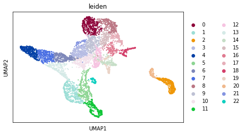
[7]:
sc.pl.umap(adata1, color="leiden")
Note that dataset 2 will be loaded later.
Computing a trajectory tree with CAPITAL
[8]:
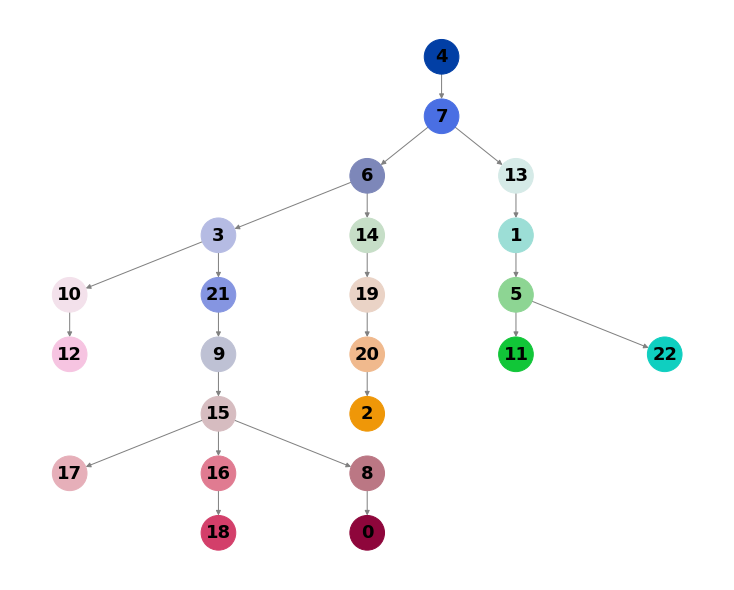
cp.tl.trajectory_tree(adata1, root_node="4", groupby="leiden", tree=None)
Draw the calculated tree.
[9]:
cp.pl.trajectory_tree(adata1)
Apply the same process to one or more datasets that you would like to align.
[10]:
adata2 = cp.dataset.velten17()
The dataset already exist in ../data/capital_dataset/velten17_capital.h5ad.
Reading datasets from ../data/capital_dataset/velten17_capital.h5ad.
[11]:
adata2
[11]:
AnnData object with n_obs × n_vars = 915 × 249
    obs: 'n_genes', 'n_counts', 'leiden'
    var: 'n_cells', 'highly_variable', 'means', 'dispersions', 'dispersions_norm'
    uns: 'diffmap_evals', 'hvg', 'leiden', 'leiden_colors', 'leiden_sizes', 'neighbors', 'paga', 'pca', 'umap'
    obsm: 'X_diffmap', 'X_pca', 'X_umap'
    varm: 'PCs'
    obsp: 'connectivities', 'distances'
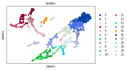
[12]:
sc.pl.umap(adata2, color="leiden")
[13]:
cp.tl.trajectory_tree(adata2, root_node="0", groupby="leiden", tree=None)
[14]:
cp.pl.trajectory_tree(adata2)

Aligning trajectory trees with CAPITAL
The alignment of trajectory trees is calculated by minimizing an alignment distance. You can specify the number of highly variable genes for both of the data so that the intersection of those genes is used to calculate the tree alignment.
[15]:
cdata = cp.tl.tree_alignment(adata1, adata2, num_genes1=2000, num_genes2=2000)
Calculating tree alignment
411 genes are used to calculate cost of tree alignment.

Calculation finished.
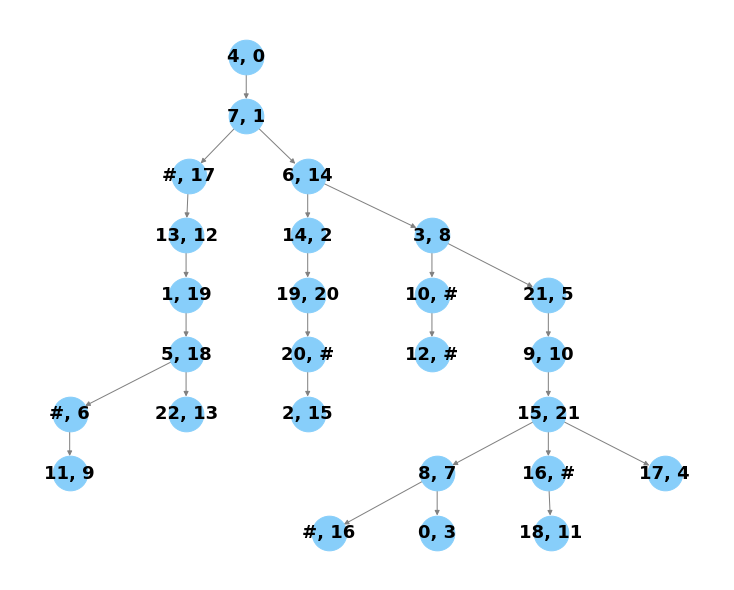
Draw the tree alignment result.
[16]:
cp.pl.tree_alignment(cdata)
[17]:
cdata.alignmentlist
[17]:
[('alignment000',
  ['4', '7', '#', '13', '1', '5', '22'],
  ['0', '1', '17', '12', '19', '18', '13']),
 ('alignment001',
  ['4', '7', '#', '13', '1', '5', '#', '11'],
  ['0', '1', '17', '12', '19', '18', '6', '9']),
 ('alignment002',
  ['4', '7', '6', '14', '19', '20', '2'],
  ['0', '1', '14', '2', '20', '#', '15']),
 ('alignment003',
  ['4', '7', '6', '3', '10', '12'],
  ['0', '1', '14', '8', '#', '#']),
 ('alignment004',
  ['4', '7', '6', '3', '21', '9', '15', '8', '#'],
  ['0', '1', '14', '8', '5', '10', '21', '7', '16']),
 ('alignment005',
  ['4', '7', '6', '3', '21', '9', '15', '8', '0'],
  ['0', '1', '14', '8', '5', '10', '21', '7', '3']),
 ('alignment006',
  ['4', '7', '6', '3', '21', '9', '15', '16', '18'],
  ['0', '1', '14', '8', '5', '10', '21', '#', '11']),
 ('alignment007',
  ['4', '7', '6', '3', '21', '9', '15', '17'],
  ['0', '1', '14', '8', '5', '10', '21', '4'])]
Aligning cells along each linear trajectory path
[18]:
cp.tl.dpt(cdata)
Run dtw (dynamic time warping) to calculate cell-cell matching.
[19]:
cp.tl.dtw(cdata, gene=cdata.genes_for_tree_align, multi_genes=True)
[20]:
cp.pl.dtw(cdata, gene=["multi_genes"], alignment=["alignment001", "alignment006"],
          data1_name="Setty+2019", data2_name="Velten+2017")

Draw expression dynamics of specified genes along respective alignments.
[21]:
main_markers = [
        ["alignment000", "ITGA2B"],
        ["alignment006", "LGMN"]
     ]
[22]:
for alignment, gene in main_markers:
    cp.pl.gene_expression_trend(
        cdata, gene=gene, alignment=alignment, fontsize=16, ticksize=16, multi_genes=True, switch_psedotime=True,
        data1_name="Setty+2019", data2_name="Velten+2017", polyfit_dimension=3
    )


Writing CAPITAL results
[23]:
cdata.write("../results/cdata")
[24]:
cdata = cp.tl.read_capital_data("../results/cdata")
Calculating similarity scores of genes in cell-cell alignment
[25]:
cp.tl.genes_similarity_score(cdata, alignment="alignment002", min_disp=0.5)
Calculating similarity score of 5148 genes in alignment002
Calculating finished
[26]:
cdata.similarity_score["alignment002"]
[26]:
array(['HN1', 'WHSC1', 'TROAP', ..., 'ARPP21', 'FCRL1', 'NBEAL1'],
      dtype=object)
See gene expression trends that have similar trends in the alignment.
[27]:
high_similarlity_genes = cdata.similarity_score["alignment002"][:4]
[28]:
cp.pl.gene_expression_trend(cdata, high_similarlity_genes, alignment="alignment002",
    data1_name="Setty+2019", data2_name="Velten+2017")

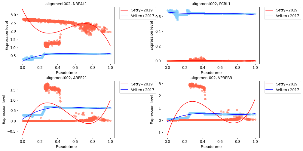
See also gene expression trends that have lower similarity scores in the alignment.
[29]:
low_similarlity_genes = cdata.similarity_score["alignment002"][::-1][:4]
[30]:
cp.pl.gene_expression_trend(cdata, low_similarlity_genes, alignment="alignment002",
    data1_name="Setty+2019", data2_name="Velten+2017")
[ ]: