Use user defined pseudotime¶

CAPITAL can now also use pseudotime that are calculated in other methods.

[1]:

import capital as cp
import scanpy as sc
import numpy as np

In this tutorial, we will use the same datasets as previous tutorial.

[2]:

adata1 = cp.dataset.setty19()

The dataset already exist in ../data/capital_dataset/setty19_capital.h5ad.
Reading datasets from ../data/capital_dataset/setty19_capital.h5ad.

[3]:

adata1

[3]:

AnnData object with n_obs × n_vars = 5780 × 1999
    obs: 'n_genes', 'leiden'
    var: 'n_cells', 'highly_variable', 'means', 'dispersions', 'dispersions_norm'
    uns: 'diffmap_evals', 'hvg', 'leiden', 'leiden_colors', 'leiden_sizes', 'neighbors', 'paga', 'pca', 'umap'
    obsm: 'X_diffmap', 'X_pca', 'X_umap'
    varm: 'PCs'
    obsp: 'connectivities', 'distances'

Calculating Diffusion Pseudotime using scanpy. This can be replaced by other methods, which can be implemented in your own preprocessing steps.

[4]:

adata1.uns['iroot'] = np.flatnonzero(adata1.obs['leiden'] == '4')[0]
sc.tl.dpt(adata1)

Now, pseudotime is stored in adata.obs

[5]:

adata1.obs

[5]:

	n_genes	leiden	dpt_pseudotime
index
Run4_120703408880541	1697	1	0.660055
Run4_120703409056541	1097	7	0.103425
Run4_120703409580963	834	8	0.614602
Run4_120703423990708	994	8	0.609378
Run4_120703424252854	2277	19	0.507636
...	...	...	...
Run5_241114589051630	2802	11	0.922035
Run5_241114589051819	1695	10	0.474332
Run5_241114589128940	2131	5	0.510828
Run5_241114589357942	2982	11	0.920328
Run5_241114589841822	2374	19	0.473308

5780 rows × 3 columns

[6]:

sc.pl.umap(adata1, color=["leiden", "dpt_pseudotime"])

../_images/tutorials_capital_tutorial_adding_pseudotime_10_0.png

Apply the same process to one or more datasets that you would like to align.

[7]:

adata2 = cp.dataset.velten17()

The dataset already exist in ../data/capital_dataset/velten17_capital.h5ad.
Reading datasets from ../data/capital_dataset/velten17_capital.h5ad.

[8]:

adata2.uns['iroot'] = np.flatnonzero(adata2.obs['leiden'] == '0')[0]
sc.tl.dpt(adata2)

[9]:

sc.pl.umap(adata2, color=["leiden", "dpt_pseudotime"])

../_images/tutorials_capital_tutorial_adding_pseudotime_14_0.png

Aligning trajectory trees¶

[10]:

cp.tl.trajectory_tree(adata1, root_node="4", groupby="leiden", tree=None)

[11]:

cp.tl.trajectory_tree(adata2, root_node="0", groupby="leiden", tree=None)

[12]:

cdata = cp.tl.tree_alignment(adata1, adata2, num_genes1=2000, num_genes2=2000)

Calculating tree alignment
411 genes are used to calculate cost of tree alignment.

Calculation finished.

Draw the tree alignment result.

[13]:

cp.pl.tree_alignment(cdata)

../_images/tutorials_capital_tutorial_adding_pseudotime_20_0.png

Applying preprocessed pseudotime for dynamic time warping¶

Specify the name of the column which stores pseudotime and the preprocessed pseudotime will be used in downstream analysis.

[14]:

cp.tl.dtw(cdata, gene=cdata.genes_for_tree_align, multi_genes=True, pseudotime="dpt_pseudotime")

[15]:

cp.pl.dtw(cdata, gene=["multi_genes"], alignment=["alignment001", "alignment006"], col_pseudotime="dpt_pseudotime",
          data1_name="Setty+2019", data2_name="Velten+2017")

../_images/tutorials_capital_tutorial_adding_pseudotime_23_0.png

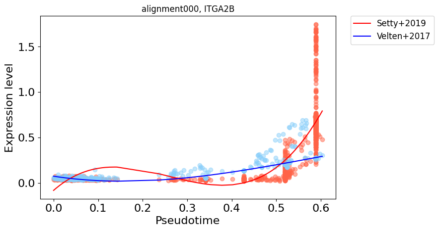
[16]:

main_markers = [
        ["alignment000", "ITGA2B"],
        ["alignment006", "LGMN"]
     ]

[17]:

for alignment, gene in main_markers:
    cp.pl.gene_expression_trend(
        cdata, gene=gene, alignment=alignment, fontsize=16, ticksize=16, multi_genes=True, col_pseudotime="dpt_pseudotime",
        switch_psedotime=True,data1_name="Setty+2019", data2_name="Velten+2017", polyfit_dimension=3
    )

../_images/tutorials_capital_tutorial_adding_pseudotime_25_0.png

../_images/tutorials_capital_tutorial_adding_pseudotime_25_1.png

[ ]: